SideFX Houdini is a tool from the visual effects industry which is used for tasks which involve procedurally generating or manipulating geometry, like simulating explosions using fluid dynamics or synthesizing a city based on geometric rules. It provides a node-based visual programming environment with a large library of common operations built in, but also makes it easy to drop in custom code using its own C-like language called Vex or Python. The networks of nodes generally flow downward, where each node is outputting modified geometry based on its inputs, so the results of operations can be aggressively cached. The usual way of working in Houdini is to build up to a result incrementally, and then when you have what you need you can render out the full, high fidelity result (images or geometry) as quickly as your available hardware allows. It’s not a tool intended for real-time effects (like Touch Designer, for example).
But what if you tried to use it in a real-time application anyway? Would that be particularly useful for anything? I know the answer is yes for at least one application: rapid-prototyping algorithms for controlling robots.
Let’s look at a simple end-to-end example of doing this with Houdini.
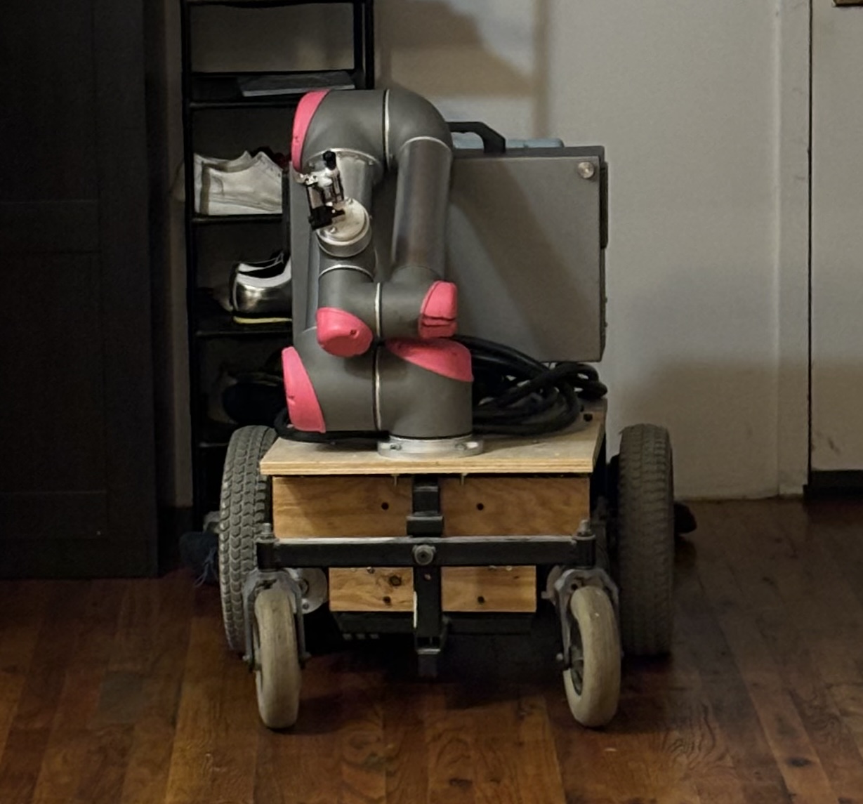
I have a mobile robotics platform I call Slug that I’ve been hacking on. It’s the bottom half of an electric wheelchair stuffed with a large DIY 18650-based LiPo battery, drive electronics, and a big inverter so I can plug in my UR5 robot arm. It’s held together with scrap plywood and hardware store parts. There are a few specific projects that I want to use it for but it’s also just an excuse to try solving various robotics problems myself.
One of those problems is motion planning. Let’s say I wanted Slug to go over to an object and pick it up. It needs to be able to figure out where it is relative to the object and then navigate to it through an environment that might have various obstacles. An old, intuitive, and easy to implement means for accomplishing this is known as the dynamic window approach.
The basic idea of is to generate (dynamically) a bunch of paths (a window) that the robot could follow from the place where it currently is, then compute costs for them based on how “good” they are, and finally pick the one that has the lowest cost. The robot can then follow that path for a little while before repeating the process to adjust its path. Optimization-based approaches like this can be very pleasant to work with because they allow for a smooth creative space. You can start out with a naive approach for each part and get something that sort of works, then replace it in bits and pieces to incrementally improve. Plus it gives you a few knobs that you can turn to explore solutions, like the relative scales of your costs or how long the candidate paths you generate are, or how often you run the process to update your plan.
Slug is what is called a differential wheeled robot - it moves forward if the wheels turn together and if they rotate at the same speed opposite each other then it turns in place. A simple way to think about generating the candidate paths is to imagine that we take the speeds that the robot is currently turning the wheels and just calculate the path that the robot would take if those speeds were fixed at slightly different values. That path will look like an arc. Sweep across a range of speeds and you’ll have a collection of candidate arc paths that the robot could follow in the near future. Then to score them you can walk along each and see how far away the robot is from obstacles and the goal at every point. Being close to an obstacle or being far from the goal adds cost to the path. Then you just pick the candidate path with the lowest total cost and that gives you the new speed for each of the wheels.
What does an implementation of this look like in Houdini?
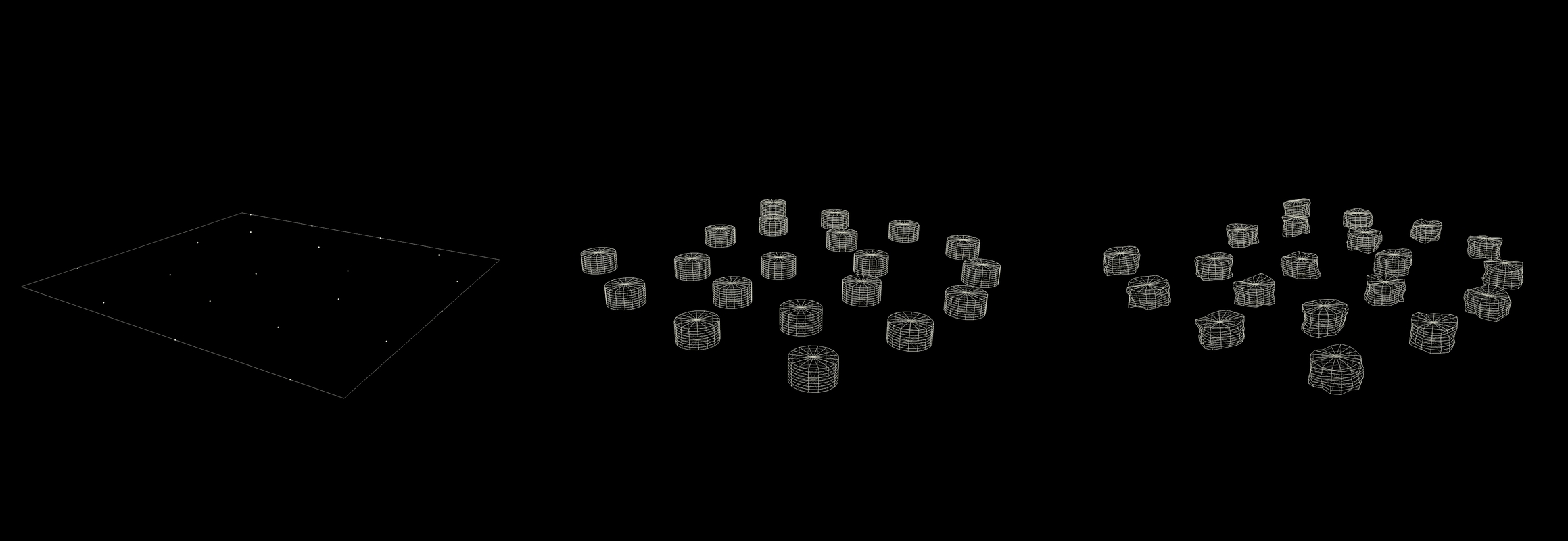
First, to set up the problem I needed some obstacles. I made a square and scattered some points on it. I copied a cylinder onto each of the points and then shifted the points in all these cylinders by a noise function just for fun.
Then I needed a point for where the robot would start in the scene and a point for where the robot should end up (the goal). I set a 4 element vector attribute on the robot point and assigned it a quaternion orientation so I could keep track of what direction the robot was pointing in. I used photogrammetry to 3D scan Slug’s wheeled base and copied that model onto this point. The goal got an X.
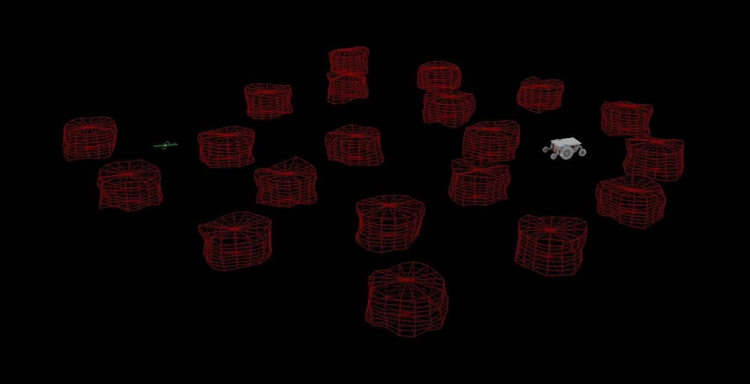
There is some information about the robot that will be needed to know how to move it and to generate the paths in each window. For that I attached a few more attributes to note down the radius of the wheels, their physical separation, and their current rotational velocity.
That’s all that is needed to be ready to implement the algorithm.
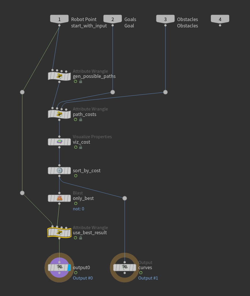
Here is the network which handles one iteration of the algorithm. As a reminder in case you’re not familiar with Houdini, geometry flows downward through these nodes and each one makes some modifications to it that are passed further along. At the top are inputs for the point representing the robot with the information about it attached, a point representing the goal position, and points representing the positions of obstacles.
The gen_possible_paths node is responsible for looking at the current velocities of the robot’s wheels and the
physical information about them and using that to generate a collection of paths that could be followed by adjusting the
wheel speeds. The speeds are just swept linearly over a range relative to their current values and for each a certain
number of points along the path are computed and added to a polyline which will be included in the output of the node.
The polylines are labeled with the wheel speeds that were used to generate them, so that those can be plucked from
whichever one turns out to be the best and used to set the new wheel speeds. It’s implemented using some Vex code:
int num_candidates = chi("num_candidates");
int path_depth = chi("path_depth");
float scale = chf("scale");

// For each potential path
for (int i = 0; i < num_candidates; i++) {
    // Make a polyline to represent this candidate path
    int path = addprim(0, "polyline");

    // Get the position and heading of the robot in the XZ plane
    float x = @P.x;
    float y = @P.z;
    float heading = quaterniontoeuler(@orient, XFORM_XYZ).y;

    // Sweep the nearby available wheel speeds
    float ratio_complete = (float)i / (num_candidates - 1);
    float adj = lerp(-scale, scale, ratio_complete);
    float left = f@left - adj;
    float right = f@right + adj;

    // Step through the path
    for (int j = 0; j < path_depth; j++) {
        float v = f@wheel_r * (left + right) / 2;
        float vrot = f@wheel_r * (right - left) / f@wheel_sep;
        heading += vrot;

        x += v * cos(heading);
        y += -v * sin(heading);

        int pt = addpoint(0, set(x, 0, y));
        addvertex(0, path, pt);
    }

    // Keep track of the owner (for handling multiple robots)
    // and the wheel velocities this path corresponds to
    setprimgroup(0, "paths", path, 1);
    setprimattrib(0, "pt", path, @ptnum);
    setprimattrib(0, "left", path, left);
    setprimattrib(0, "right", path, right);
}
After generating the paths in the gen_possible_paths node we compute the costs for them in the path_costs node. This
node additionally has the goal point and the obstacles points as inputs.
// The goal position is the position of the first point
// in the third input
vector goal_pos = point(1, "P", 0);

// Final distance to the goal
int path_pts[] = primpoints(0, @primnum);
int last_pt = path_pts[len(path_pts) - 1];
vector last_pos = point(0, "P", last_pt);

float min_dist_to_goal = 1e3;
float min_dist_to_obstacle = 1e3;
for (int i = 0; i < len(path_pts); i++) {
    int pt = path_pts[i];
    vector pos = point(0, "P", pt);

    int nearest_obstacle = nearpoint(2, pos);
    vector obstacle_pos = point(2, "P", nearest_obstacle);
    float obstacle_dist = length(obstacle_pos - pos);

    if (obstacle_dist < min_dist_to_obstacle) {
        min_dist_to_obstacle = obstacle_dist;
    }

    float goal_dist = length(goal_pos - pos);

    if (goal_dist < min_dist_to_goal) {
        min_dist_to_goal = goal_dist;
    }
}

float to_goal_cost = min_dist_to_goal / (min_dist_to_goal + 1);
float obstacle_cost = chramp("obstacle_cost", min_dist_to_obstacle / chf("obstacle_influence_r"));
f@obstacle_cost = obstacle_cost;
f@cost = to_goal_cost + obstacle_cost;
A ramp channel (lookup table with a GUI) plus a float channel (slider GUI) are used to tune how the distance to the obstacles is turned into the actual cost. After we have the costs we just order the paths by them and only keep the one with the lowest cost.
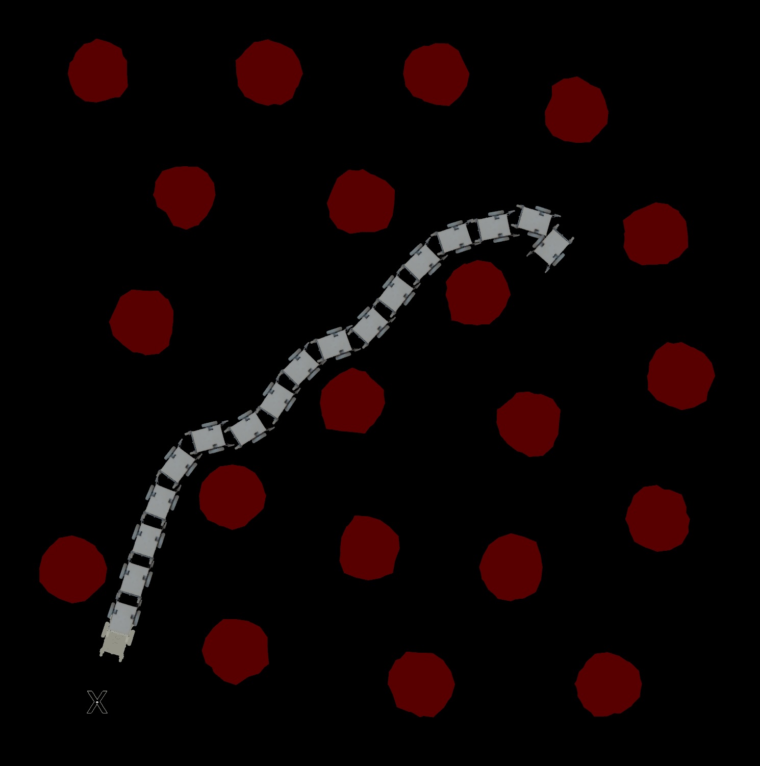
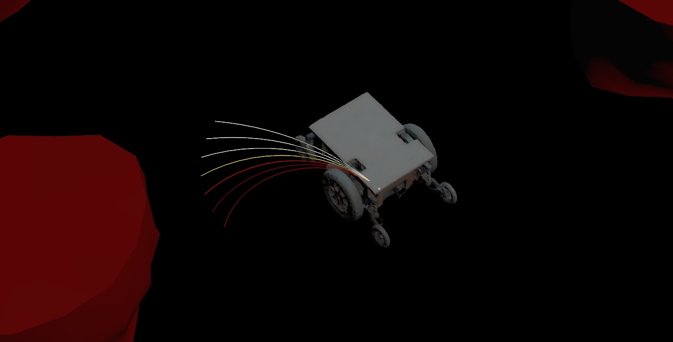
Here the candidate paths and their costs are visualized (via the viz_cost node) with higher cost paths getting darker
colors. We can see that the robot is going to end up continuing a wide turn past the obstacle to its left. The paths
that would take it into collision with the obstacle have been assigned a high cost.
The last step is to apply the wheel velocities of the lowest cost path to the robot’s state in the use_best_result
node:
int best_path = findattribval(1, "prim", "pt", @ptnum);

if (best_path == -1) {
    return;
}

f@left = prim(1, "left", best_path);
f@right = prim(1, "right", best_path);
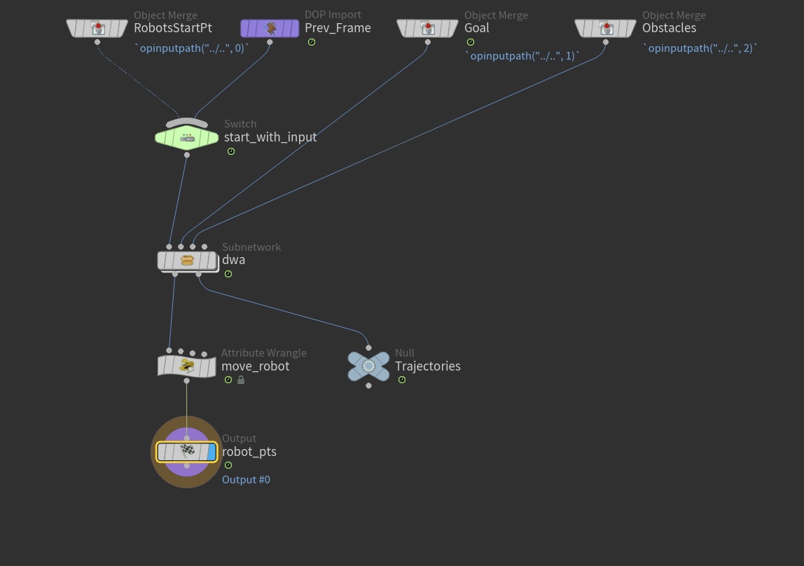
All that remains is to move the point representing the robot based on the wheel velocities (the move_robot node below)
and repeat everything over and over. In Houdini you do this with a node called a Solver, which evaluates a network and
then allows you to feed its result back into itself to compute a new output for the next frame. The network we were
looking about above is contained inside of the dwa Subnetwork node inside the Solver here:
With that, it works! At least virtually:
Now let’s do it on the real robot!
We have a new challenge to overcome if we want to do the same thing with the real robot. In the simulation we just directly compute where the robot is each frame, but with the real robot we can’t directly know where it is in space relative to the goal point. We need some way to capture its location and inject that into Houdini.
Because this is just an experiment for learning and fun I decided to cheat and use a Vive Tracker, which is a 6 DoF motion tracker that uses the Lighthouse tracking system from the Vive. It’s relatively easy to use Python to stream high speed and accurate position and orientation data from the tracker. The more fiddly aspect is getting that data stream into Houdini. Even though at the start I explained how Houdini is not really meant for real-time applications, it actually does have some functionality that explicitly supports it inside of a special kind of network called a CHOP network.
CHOPs = Channel Operators. They work very similar to the Surface Operators (SOPs) that I showed for manipulating geometry in the sections above. But CHOPs are intended for manipulating time-series sequences like animation data or audio. They support recording inputs from the user or external systems to use to drive animations. But it’s implemented in a flexible way that let’s you use it pretty much anywhere you would like to.
For pulling in the Vive Tracker data I made CHOP network with a Pipe In node with its source set to network. There’s a somewhat clunky network protocol that can be used to stream data from external software into this node. I slapped together some Python code for sending in values this way. Then I wrote some more Python code to plug in the tracker data. After that it was short work to get a model of the tracker to follow the real one in Houdini:
I attached the Vive Tracker to the UR5 and then added a few more nodes to get my virtual robot to have an offset that matched the real offset between the base and the Vive Tracker. Then when I moved the real Vive Tracker around my apartment I saw the virtual robot follow the same motion. With that the problem of letting Houdini know where the robot is was solved.
What remained was to take the wheel velocities computed in Houdini and make it so the actual robot used them. Houdini lets you drop down a Python node and run arbitrary code so this task was pretty straightforward. I dumped the wheel velocity values into some JSON and spat that over the network to another Python script running on a computer on the robot which then wrote them to the motor controller, making the actual wheels turn.
At this point there are no more challenges to overcome. I set up a chair as a real world obstacle and made a point in Houdini to mark its position, which was fed into the network in place of the original scattered points I used initially. I adjusted the goal point to a real world location some distance from the robot. Then I just hit play in Houdini and let it do its thing:
I’m writing about it now but I did this project back in the first week of January 2025.